Lissajous Curves: Where Mathematics Meets Music and Light

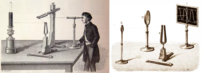
Obviously, it all begins with two physicists

The curves we call "Lissajous" actually have an earlier origin. In 1815, American mathematician Nathaniel Bowditch first described these patterns while studying pendulum motion, which is why some prefer the name Bowditch curves.

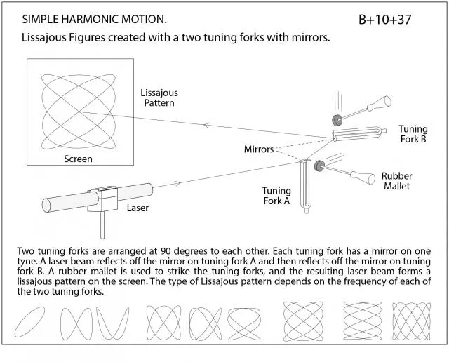
But it was French physicist Jules Antoine Lissajous who, in the 1850s, turned them into spectacle. His experiment was simple: mirrors attached to vibrating tuning forks, projecting beams of light onto screens in darkened lecture halls. Audiences could watch sound become "visible". The curves took his name and have remained scientifically useful ever since.

The Mathematics

A Lissajous curve appears when two perpendicular oscillations combine. The equations are quite simple:

\[ \begin{cases} X = A_x \cos(2\pi f_x t + \phi_x) \\ Y = A_y \cos(2\pi f_y t + \phi_y) \end{cases} \]

Where:

• \(A_x\) and \(A_y\) control amplitude (the size in each direction)
• \(f_x\) and \(f_y\) are the frequencies of oscillation (in Hz)
• \(\phi_x\) and \(\phi_y\) are the phase offsets
• \(t\) is time

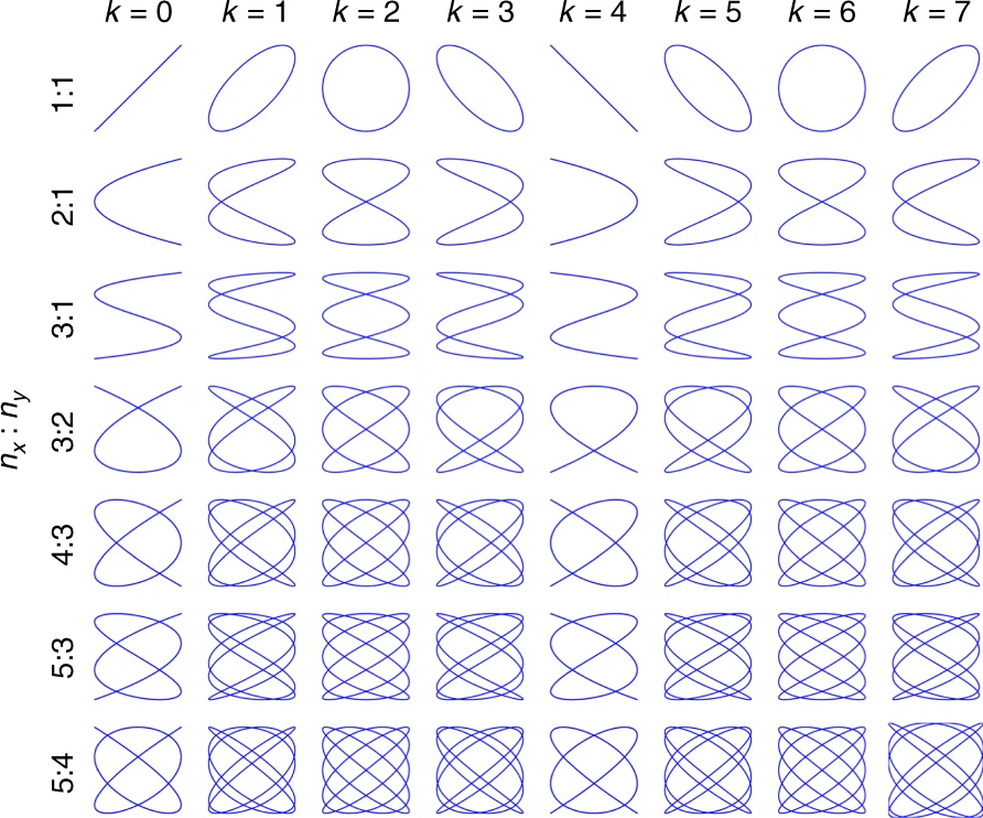
Frequency Ratios and Periodicity

If both frequencies share a greatest common divisor \(f_0\), we can write:

\[ \frac{f_x}{f_y} = \frac{n_x f_0}{n_y f_0} = \frac{n_x}{n_y} \]

where \(n_x\) and \(n_y\) are coprime integers. This ratio determines everything about the curve's structure. The value \(f_0\) becomes the frame rate; the frequency at which the entire pattern repeats. In other words, every \(1/f_0\) seconds, the trajectory traces exactly the same path.

Simple ratios produce closed curves. Irrational ratios create paths that wander eternally without repeating, gradually filling their bounds.

The Phase Parameter \(k\)

The combined effect of both phase offsets can be captured in a single parameter \(k\), defined as:

\[ k = \frac{4}{\pi}(n_x \phi_y - n_y \phi_x) \]

This parameter has a period of 8, meaning \(k\) and \(k + 8\) produce identical figures. When \(k\) is an integer, eight distinct basic figures exist for any given frequency ratio.

Assuming \(n_x > n_y\) and setting \(\phi_x = 0\), the equations simplify to:

\[ \begin{cases} X = A_x \cos(2\pi n_x f_0 t) \\ Y = A_y \cos\left(2\pi n_y f_0 t + \dfrac{k\pi}{4n_x}\right) \end{cases} \]

The figure below shows how \(k\) affects the trajectory for various frequency ratios. Notice that when \(k = 2\) or \(k = 6\), the figures achieve maximum symmetry: symmetric about both axes and the origin simultaneously.

Symmetry Properties

The symmetry of a Lissajous figure depends on the parity of \(n_x\) and \(n_y\):

• When \(n_x\) is even → symmetric about the \(x\)-axis
• When \(n_y\) is even → symmetric about the \(y\)-axis
• When both are odd → symmetric about the origin

Two Lissajous patterns with parameters \((n_x, n_y, k)\) and \((n_x', n_y', k')\) are identical if and only if:

\[ n_x' = n_x, \quad n_y' = n_y, \quad k' = k + 8m \]

where \(m\) is any integer.

Fill Factor: Measuring Trajectory Density

A critical property for applications is the fill factor (FF); a measure of how densely the curve covers its bounding rectangle. Lissajous trajectories are characteristically dense at the edges and sparse near the center. The maximum gap appears in an approximate parallelogram containing the origin.

For scanning applications like LIDAR, minimizing this gap (maximizing density) is essential. Research has shown that \(k = 2\) produces optimal density for most frequency ratios, establishing a key design rule for Lissajous-based systems.

Seeing Sound: The Music Connection

Here's where Lissajous curves become almost magical: those frequency ratios are musical intervals.

When two notes form a consonant harmony, their Lissajous figure is clean, closed, symmetrical. Dissonance produces chaos: curves that refuse to settle.

You can literally see whether two notes sound good together.

This isn't coincidence. Musical harmony is, at its core, a relationship between frequencies. Lissajous curves simply make that relationship visible.

Making Your Own

The Victorian Way: Harmonographs

Before computers, there were harmonographs: pendulum-driven drawing machines popular in the 1800s. Two or more pendulums swing in perpendicular directions, and a pen traces their combined motion onto paper.

Simple Experiments

• Sand pendulums: A funnel of sand swinging over paper
• Laser on speakers: Mount a mirror on one speaker cone, bounce a laser off it onto a wall, play two frequencies through stereo speakers (similar to how Lissajous did it)
• Oscilloscope: Feed two audio signals into \(X\) and \(Y\) inputs (easy to do and actually useful)

The Modern Way: Code

A few lines in Python, Processing, or p5.js will generate infinite variations:

import numpy as np
import matplotlib.pyplot as plt

t = np.linspace(0, 1, 10000)
nx, ny = 5, 4
k = 2
f0 = 1

x = np.cos(2 * np.pi * nx * f0 * t)
y = np.cos(2 * np.pi * ny * f0 * t + k * np.pi / (4 * nx))

plt.plot(x, y)
plt.axis('equal')
plt.show()

Play with nx, ny, and k. Watch the curves transform.

Applications

Science and Engineering

Oscilloscopes have used Lissajous figures since the early 20th century to compare signal frequencies. An unknown frequency fed into one axis, a known reference into the other. The resulting shape instantly reveals their ratio and thus the unknown frequency.

MEMS LIDAR and Laser Scanning

Modern microelectromechanical systems (MEMS) scanning mirrors exploit Lissajous trajectories for solid-state LIDAR systems. By driving a two-axis mirror with sinusoidal waveforms at carefully chosen frequencies, engineers create scanning patterns that cover a field of view with predictable density and timing.

The design rules are precise:

1. Frame rate is determined by \(f_0\) (the GCD of driving frequencies)
2. Phase parameter \(k = 2\) ensures maximum symmetry and optimal coverage
3. Spatial resolution depends on \(n_x\) and \(n_y\): higher values yield denser trajectories

That enables various applications from autonomous vehicle sensing to 3D imaging microscopy.

Art and Design

Perhaps the most famous Lissajous figure hidden in plain sight: the ABC television logo, a stylized \(1:3\) ratio curve that has represented the network since 1965.

More recently, Meta's 2021 rebrand introduced a logo that is essentially an infinite loop: a Lissajous-like figure rotated in 3D space, representing connection and infinity.

Beyond Two Dimensions

Lissajous Knots

Add a third oscillation:

\[ Z = A_z \cos(2\pi f_z t + \phi_z) \]

Now the curve spirals through 3D space. Depending on the frequency ratios, it can form true mathematical knots: curves that loop through themselves in ways that cannot be untangled without cutting.

These Lissajous knots have become a subject of serious topological study.

Related Patterns

• Spirograph toys produce related curves called hypotrochoids and epitrochoids
• Certain orbital mechanics problems produce figure-eight trajectories that echo Lissajous geometry
• Lissajous orbits in space (around Lagrange points) share the name, though the mathematics differs

Living Curves

Maths tends to be pretty abstract. The more you study it, the less visual it becomes. Lissajous curves change that. They straight up ask to be experienced.

Try the online generator I built and play with the parameters by yourself.

Open in fullscreen by clicking here